Introduction

SeqNjoy is a stand-alone application designed to generate and analyze differential gene expression results from RNA-Seq experiments.

This Quick Guide is intended to help you perform an RNA-Seq data analysis using SeqNjoy. For a complete description of SeqNjoy and its functionalities, please refer to the SeqNjoy Tutorial.

At https://bioinfogp.cnb.csic.es/files/samples/rnaseq/, you will find information about the experiment from which the data used in this example was obtained. On that link, you can also download all the files used in this guide, allowing you to perform the suggested RNA-Seq data analysis with SeqNjoy on your own.

In summary, the project includes nine sample files of Saccharomyces cerevisiae short reads as input. As described in the Content section of the link, three groups of replicates were grown under three different CO2 and pH conditions (“pH5_CO2”, “pH5”, and “pH3”).

In the project titled “S. cerevisiae pH CO2,” analyzed in this guide, two comparisons between conditions will be performed: “pH5_CO2” versus “pH5” and “pH3” versus “pH5”.

Step-by-Step Guide

1. Choose a Project Folder location on your computer or an external drive. New projects will be created inside this directory. Then, type the project name (S. cerevisiae pH CO2) in the text box at the bottom of the Homepage and click Start New Project (Figure 1).
   
   
   

   Figure 1: Creating your project

2. On the Project’s Main Page (Figure 2), click Load Files and select the short-read (FASTQ) files from your computer.
   
   
   

   Figure 2: Project’s Main page

3. The application will display a pop-up window showing the upload progress (Figure 3).
   
   
   
   

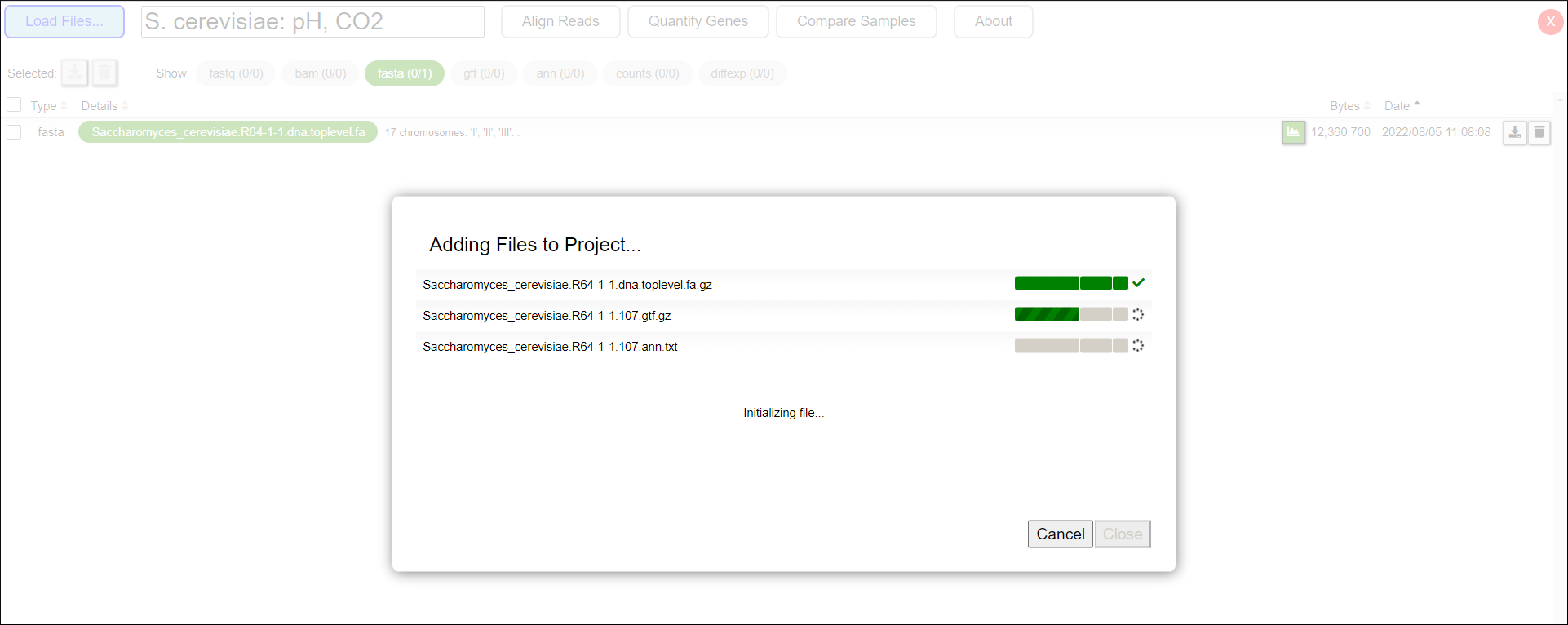
   Figure 3: Uploading files in SeqNjoy

   
   Once the files have been added to the project, a message stating “All steps done!” will appear (Figure 4). Click the Close button to return to the Project’s Main Page.
   
   
   

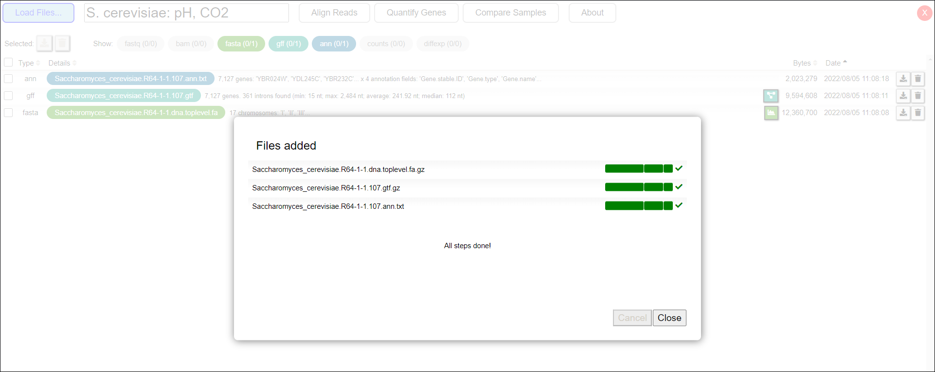
   Figure 4: Uploading process successful

4. After the files have been added, the Project’s Main Page will now list all 18 files included in the project (Figure 5). Note that paired-end files are automatically recognized and grouped as pairs in the same row.
   
   
   

   Figure 5: File List

All FASTQ files contain one million reads. For this example, we have randomly subset this amount of short reads from the real files to improve processing speed.

5. Download the reference genome (FASTA) file and gene features (GFF) file. Click the “Download Genomes” button on the Project’s Main Page, then select “Download Genomes from Ensembl” (Figure 6) to open the download dialog.
   
   
   

   Figure 6: Selecting Download Genomes from Ensembl task

6. Select the taxonomic group “Fungi”, then choose Saccharomyces cerevisiae (Saccharomyces cerevisiae) and click Check Genome Availability. If Ensembl is online and reachable, the dialog will display the available files (Figure 7). Check “Sequence (FASTA)” and “Annotations (GFF3)”, then click Download!.
   
   
   

   Figure 7: Download Genomes: selecting taxonomic group and species, checking avalaibility and choosing files for download

7. The application will display a pop-up window showing the progress of the file download (Figure 8). Once the files have been added to the project, a message stating “All steps done!” will appear (Figure 4). Click the Close button to return to the Project’s Main Page.
   
   
   

   Figure 8: Download Genomes: All files have been downloaded and processed

8. The Project’s Main Page now includes the two downloaded files (Figure 9).
   
   
   

   Figure 9: File List including downloaded genome files

9. Click the icon in the rightmost column of the GFF file row under “Details” to visualize the genome structure as a hierarchical tree showing the dependencies between feature types in the GFF file (Figure 10).
   
   
   

   Figure 10: Viewing the tree of dependencies between the feature types present in the GFF file

10. Perform Quality Control (QC) on one of the short-read file pairs. Click the “Quality Control” button on the Project’s Main Page and select “Quality Control with fastp” (Figure 11).
    
    
    

    Figure 11: Selecting Quality Control with fastp task

11. In the Quality Control of Reads dialog, select the input FASTQ file. When selecting the first read of the pair (e.g., 1M_SRR9336476_1.fastq.gz) as “Fastq 1”, its corresponding partner will automatically be selected as “Fastq 2” (Figure 12). Click the Launch! button to start the quality control process.
    
    
    

    Figure 12: Quality control of Reads: Selecting input FASTQ files and specifying the number of reads to include in the QC process

12. Once the process is complete, close the dialog. On the Project’s Main Page, the icon in the rightmost column of the selected FASTQ pair will be enabled. Clicking this icon opens the QC report (Figure 13), where users can review metrics and visualizations related to read quality. For a detailed breakdown of the Quality Control Report’s contents, refer to the Quality Control Report section in the SeqNjoy Tutorial.
    
    
    

    Figure 13: Quality control report: Report begins with the summary stats and sequence quality boxplots.

13. Apply preprocessing to the FASTQ files to remove adapter fragments, trim low-quality bases, and discard reads that do not meet quality or length thresholds. Click the “Preprocess Reads” button on the Project’s Main Page and select “Preprocess Reads with fastp” (Figure 14).
    
    
    

    Figure 14: Selecting Preprocess Reads with fastp task

14. In the Preprocess Reads dialog, select all input FASTQ pairs and set the output prefix as “FILT”. This prefix will be added to the processed FASTQ filenames to distinguish them from the original files. Click the Launch! button to start preprocessing (Figure 15).
    
    
    

    Figure 15: Preprocess Reads: Selecting input FASTQ files and the adapter removal, filtering and trimming parameters

15. Once the process is complete, close the dialog. The Project’s Main Page now includes all the preprocessed files, with reads removed or trimmed according to the specified parameters (Figure 16).
    
    
    

    Figure 16: File List

    The files used in this quick guide contain reads with low adapter content and good quality values, so the number of reads removed will be minimal (Figure 17).
    

    Figure 17: Quality control report of filtered file: Note that, even for good quality input files,some reads have been removed or trimmed.

16. Now, we will align the short reads from the FASTQ files to the reference genome in the FASTA file and generate alignment files (BAM files). On the Project’s Main Page, click the Align Reads button at the top of the page (Figure 18). A submenu will appear, allowing you to choose one of the two available alignment methods in SeqNjoy. For this project, select “hisat2” by clicking “Align reads with hisat2”.
    
    
    

    Figure 18: Align Reads: selecting alignment method (aligner)

17. In the Align Reads to Genomes dialog (Figure 19), select the input FASTA and preprocessed FASTQ files. The dialog also contains various parameters related to the alignment method (shaded area on the right). For this example, select only the GFF file to account for annotated introns during alignment. Click the Launch! button to start the alignment process (Figure 20).
    
    
    

    Figure 19: Align Reads to Genomes dialog

    

    Figure 20: Align Reads to Genomes dialog ready to launch the alignments processes.

18. Alignment may take a significant amount of time, depending on the number and size of the FASTQ files. A pop-up window will show the progress of the alignment task. When the alignment process is complete, click the Close button (Figure 21).
    
    
    

    Figure 21: Alignment process ended OK

19. The Align Reads to Genomes dialog will reappear (Figure 22). Here, you can configure additional alignments if needed or click the “X” icon to close the window. Since we do not need to align more FASTQ files, click the “X” icon.
    
    
    

    Figure 22: Align Reads to Genomes dialog: click the X icon (top right) to exit the window

20. You will return to the Project’s Main Page, which will now display the newly generated alignment files (BAM files) in the File List (Figure 23). To visually explore a BAM file, click the icon in the File List for the BAM file of interest (e.g., “pH5-Rep1.bam” in Figure 23).
    
    
    

    Figure 23: Selecting a .bam file in the File list to access IGV viewer

21. You will be directed to IGV, a widely used genome browser for inspecting alignments and other genomic data. As shown in Figure 24, two tracks are loaded:
    • The upper track represents the Saccharomyces cerevisiae reference genome (chromosomes I, II, III, etc.).
      
    • The bottom track shows the alignments from the “pH5-Rep1.bam” file.
      
      
      

      Figure 24: pH5-Rep1.bam alignments file loaded in IGV

22. Select the corresponding GFF file for the BAM file in the Select GFF drop-down menu at the top. The GFF track will then be added (Figure 25).
    
    
    

    Figure 25: GFF selection

23. Zoom in on a specific genomic region to inspect the alignments. In the text box next to the GFF filename, enter the following region of chromosome I: I:126,500-136,000 (Figure 26). At this magnification, you can observe variations in read coverage between genes, reflecting differences in expression levels. Additionally, note how read colors indicate sequencing strand orientation:

    • Genes oriented forward (“> > >” in the gene bar) are colored blue.
      
    • Genes oriented in reverse (“< < <”) are colored red.
    This color-coding suggests that the sequencing protocol used was reverse stranded. For more details on strand specificity in RNA-Seq and how to determine strand orientation using IGV, refer to the Tutorial.
    
    
    

    Figure 26: Zooming in on region I:126,500-136,000 to explore the alignments on that region

24. Often, we need to compare alignments across different samples in a specific genomic region. In this example, we will load additional BAM files to visualize multiple alignments in the previously defined chromosome I region.
    To do this, select the BAM files of interest in the top Select BAM drop-down menu. Figure 27 shows an example where three additional samples (“pH5-Rep2.bam”, “pH5-CO2-Rep1.bam”, and “pH5-CO2-Rep2.bam”) have been loaded.
    
    
    

    Figure 27: Comparing alignment files with IGV

    For instance, differences in coverage (i.e., the number of reads mapped to a given region, represented by the “mountain” peaks above the reads) can be observed for the CYS3 gene between the “pH5” replicates (top) and the “pH3” replicates (bottom). Whether these differences are statistically significant can only be determined through the Compare Samples process in the following steps.

25. After inspecting the alignments, close the IGV tool by clicking the “X” icon at the top right to return to the Project’s Main Page and proceed to the next step in the workflow.
26. Click the “Quantify Genes” button on the Project’s Main Page and select “Quantify Genes with featureCounts” (Figure 28) to open the gene quantification dialog (Figure 29).
    
    
    

    Figure 28: Selecting Quantify Genes task

    

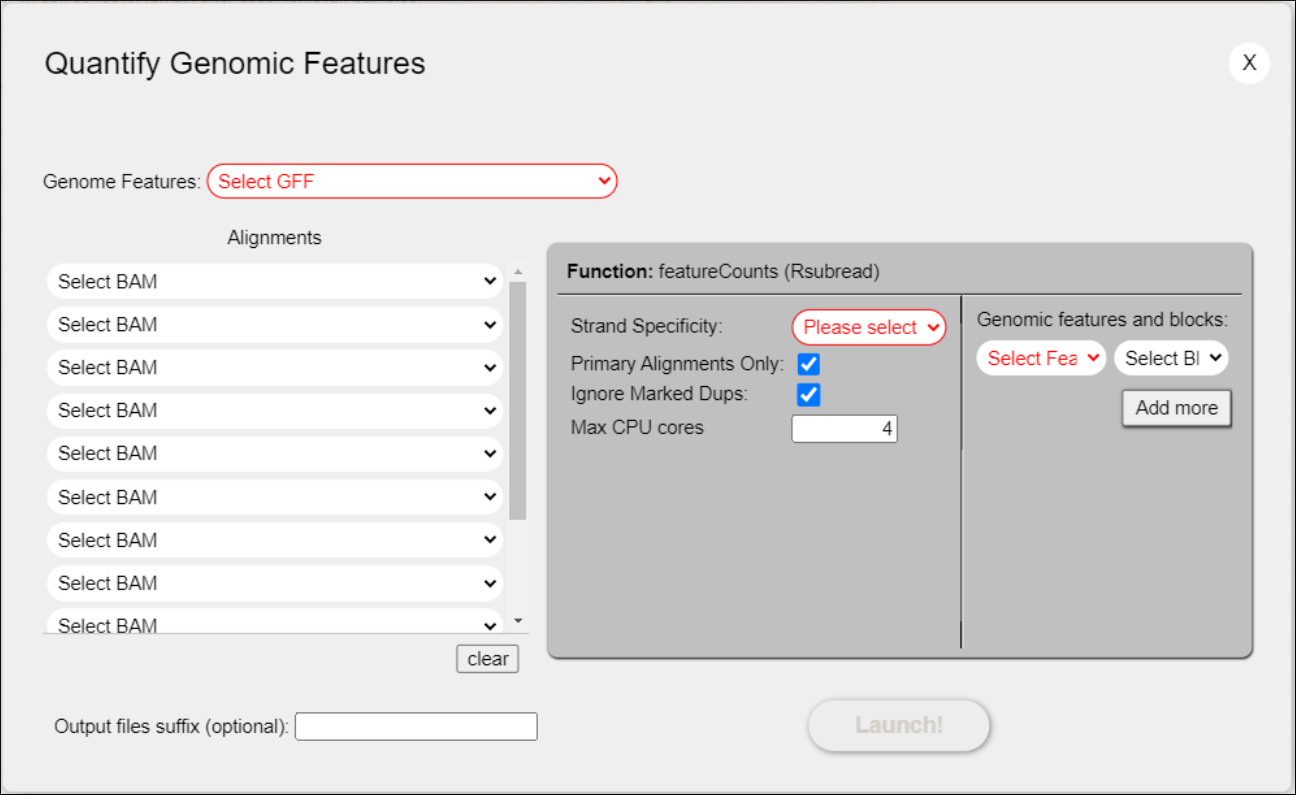
    Figure 29: Quantification dialog

27. Select the Genome Features file (GFF) from the list of loaded GFF files displayed in the drop-down menu (Figure 30).
    
    
    

    Figure 30: Select GFF file

28. Select the Alignments files (BAM) from the list of BAM files generated in the previous Align Reads task (Figure 31).
    
    
    

    Figure 31: Select BAM files

29. Open the drop-down menu labeled Strand Specificity to display the available options for this parameter (Figure 26). Strand Specificity refers to the protocol (reverse, direct, or unstranded) used in the library preparation of the samples. See the Tutorial for more insights into this important issue. In this example, a reverse stranded protocol was used, so select this option from the list.
    
    
    

    Figure 32: Select the Strand Specificity protocol used in the library preparation of the samples

30. Click “Launch!” to quantify counts-by-gene in each of the nine alignment (BAM) files. A pop-up window will display the progress of the quantification task. When the process is complete, a “done” message will be displayed. Click the Close button (Figure 33).
    
    
    

    Figure 33: Quantify Samples ended OK

31. You will return to the Quantify Genomic Features dialog. Click the “X” icon to close this window (Figure 34).
    
    
    

    Figure 34: Click the X icon (top right) to close Quantify Genomic Features dialog

32. You are now back on the “Project’s Main Page”. The File List will have been updated to include the new “counts” files generated by the quantification task (Figure 35).
    
    
    

    Figure 35: File list with the new counts (.counts) files added

33. On the Project’s Main Page (Figure 36), press Load Files and select the annotations (ANN) file from your computer. A loading dialog will appear as the file uploads. Once the upload is complete, click the Close button to return to the Project’s Main Page. You will see the new file added to the project.
    
    
    

    Figure 36: File List

34. In the following steps, you will obtain the list of differentially expressed genes between the test group of samples grown at pH5 in the presence of CO2 and the control group, which grew at pH5 in the absence of CO2. To access this task, click the Compare Samples button located at the top of the “Project’s Main Page”. Then select “Compare samples with DESeq2” as the method to perform the differential expression calculations (Figure 37).
    
    
    

    Figure 37: Compare Samples: selecting the method for calculating differential expression

35. After selecting the method, the Calculate Differential Expression dialog will appear for you to fill in (Figure 38).
    
    
    

    Figure 38: Calculate Differential Expression dialog as displayed initially.

36. Select the Counts group from the list displayed in the drop-down menu (Figure 39). The name of the Counts Group consists of two parameters chosen when quantifying genes: the name of the GFF file (Saccharomyces_cerevisiae-R64-1-1.59.gtf) and the feature type (gene).
    
    
    

    Figure 39: Calculate Differential Expression: select counts group

37. Select the counts files corresponding to the Case group of samples and the counts files corresponding to the Control group of samples from the drop-down menus. Enter identifying names for each condition in the Case Label (type “pH5_CO2”) and Control Label (type “pH5”) text boxes (Figure 40). These names will be included in the final result files.
    
    
    

    Figure 40: Calculate Differential Expression: counts files assignment to counts groups and Case and Control naming

38. We previously loaded an annotations file with useful information (annotations) that can be added to each gene in the results file containing the differential expression calculations. Select this annotations file from the Annotations drop-down menu (Figure 41). Then, launch the Calculate Differential Expression process by clicking the Launch! button.
    
    
    

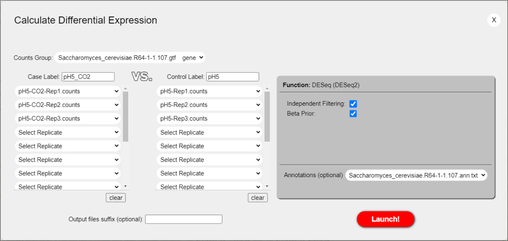
    Figure 41: Calculate Differential Expression dialog for differential expression ready to be launched

39. When the process ends, the message “done” is displayed in the pop-up window that informs you of the progress of the “differential expression” task (Figure 42).
    
    
    

    Figure 42: ph5_CO2 versus pH5 comparison ended OK

40. Click the Close button, and you will return to the Calculate Differential Expression dialog (Figure 43).
    
    
    

    Figure 43: Calculate Differential Expression dialog after returning from a previous done comparison

41. Now, we can fill in the form again to perform a new comparison between two groups of samples to calculate the differential expression between them. For example, we wish to compare the samples that grew at pH3 with those that grew at pH5. Therefore, we will consider pH3 as the “Case” condition and keep pH5 as the “Control” condition. To modify the form for the new comparison, first clear the previous “Case” data from the form by clicking the “Clear” button located at the bottom of the “Case” column (Figure 44).
    
    
    

    Figure 44: Calculate Differential Expression: using the Clear button to clean data from the dialog

42. Fill in the “Case” column with the data corresponding to the “pH3” condition, i.e., the counts files of the samples in the “pH3” condition, and provide a “Case Label” (type “pH3”) to identify this condition (Figure 45).
    
    
    

    Figure 45: Calculate Differential Expression dialog for differential expression ready to be launched for the second comparison

43. Click the “Launch!” button. After calculating the differential expression for this second comparison, the pop-up progress window will display the “done” message (Figure 46). Click the “Close” button to return to the Calculate Differential Expression dialog.
    
    
    

    Figure 46: Calculate Differential Expression for pH3 versus pH5 comparison ended OK

44. As we do not wish to perform more comparisons, click the “X” icon to close the Calculate Differential Expression window. You will then return to the Project’s Main Page, which will have been updated to list the differential expression files generated in Excel format (extension .xlsx) containing the results of the differential expression calculations for the two comparisons performed (Figure 47).
    
    
    

    Figure 47: File list with the new differential expression files (.xlsx) added

45. You can now graphically inspect any results file containing the comparison of gene expression between two conditions by using the FIESTA 2.0 analytic tool. Let’s select the file with the comparison of “pH3” versus “pH5” conditions. Click the icon located at the rightmost end of the Details column for the corresponding results (.xlsx) file (Figure 48) to access FIESTA 2.0.
    
    
    

    Figure 48: Selecting a differential expression file in the File list to access FIESTA 2.0

46. FIESTA 2.0 is an interactive tool for data visualization and filtering. The initial screen displays an MA-plot by default (Figure 49), representing Log2BaseMean values on the X axis and Log2Ratio(Case/Control) (also known as log2(FoldChange(Case/Control))) on the Y axis.
    
    
    

    Figure 49: FIESTA 2.0 window for the pH3 versus pH5 comparison

47. With FIESTA 2.0, you can apply filters to select significant genes that are differentially expressed between the two conditions. Simply type the filter criteria in the text boxes located at the top of the corresponding columns. For example (Figure 50), type “>0” in the Log2Ratio column header and “<0.05” in the “P-adjusted” column header, then press Enter to select only the 383 genes that are overexpressed in the case condition (pH3) compared to the control condition (pH5) for a significance threshold (adjusted P) of 0.05.
    
    
    

    Figure 50: FIESTA 2.0 window for the pH3 versus pH5 comparison

48. Apply a second filter to select only the underexpressed genes. Click the “All values” row to apply the filter to all genes, then type “<0” in the Log2Ratio column header and “<0.05” in the “P-adjusted” column header to select only the 102 genes that are underexpressed in the case condition (pH3) compared to the control condition (pH5) for a significance threshold (adjusted P) of 0.05 (Figure 51).
    
    
    

    Figure 51: FIESTA 2.0 window for the pH3 versus pH5 comparison

49. Take a closer look at the overexpressed genes. By clicking on the row named after its filter (Log2Ratio(pH3/pH5) > 0 AND P-adjusted <0.05), you will see the set of genes in the table. Click on the P-adjusted column header to sort the table in ascending or descending order by this value (Figure 52). Inspecting the sorted list of overexpressed genes, you will easily notice that HPF1 is clearly overexpressed (Log2Ratio=4.98) in the test (pH3) condition compared to the control (pH5) condition, and that the overexpression is statistically significant (P-adjusted=4.57·10^-92).
    
    
    

    Figure 52: FIESTA 2.0 window for the pH3 versus pH5 comparison

FIESTA 2.0 is a very versatile tool that allows users to create interactive plots that can be downloaded as high-resolution images, filter results, and export the data as tables. To learn more about all the possibilities, please refer to the SeqNjoy Tutorial.

SeqNjoy: Complete RNA-Seq workflows in your Desktop. Developed by BioinfoGP CNB-CSIC (2022)